import matplotlib.pyplot as plt
import numpy as np
import sympy as sy

sy.init_printing()
There are many new terminologies in this chapter, however they are not entirely new to us.
Let \(V\) and \(W\) be vector spaces. The mapping \(T:\ V\rightarrow W\) is called a linear transformation if an only if
\[ T(u+v)=T(u)+T(v)\quad \text{and} \quad T(cu)=cT(u) \]
for all \(u,v\in V\) and all \(c\in R\). If \(T:\ V\rightarrow W\), then \(T\) is called a linear operator. For each \(u\in V\), the vector \(w=T(u)\) is called the image of \(u\) under \(T\).
Parametric Function Plotting
We need one tool for illustrating linear transformation.
We want to plot any line in vector space by an equation: $p = p_0+tv $. We need to know vector \(p_0\) and \(v\) to plot the line.
For instance, \(p_0 = (2, 6)\), \(v=(5, 3)\) and \(p = (x, y)\), subsitute them into our equation \[ \left[ \begin{matrix} x\\y \end{matrix} \right]=\left[ \begin{matrix} 2\\6 \end{matrix} \right]+ t\left[ \begin{matrix} 5\\3 \end{matrix} \right] \]
We will create a plot to illustrate the linear transformation later.
def paraEqPlot(p0, v0, p1, v1):
    t = np.linspace(-5, 5)

    ################### First Line ####################
    fig, ax = plt.subplots(figsize=(10, 10))

    # Plot first line
    x = p0[0, 0] + v0[0, 0] * t
    y = p0[1, 0] + v0[1, 0] * t
    ax.plot(x, y, lw=3, color="red")
    ax.grid(True)
    ax.scatter(p0[0, 0], p0[1, 0], s=150, edgecolor="red", facecolor="black", zorder=3)

    # Plot second line
    x = p1[0, 0] + v1[0, 0] * t
    y = p1[1, 0] + v1[1, 0] * t
    ax.plot(x, y, lw=3, color="blue")
    ax.grid(True)
    ax.scatter(p1[0, 0], p1[1, 0], s=150, edgecolor="red", facecolor="black", zorder=3)

    # Set the position of the spines
    ax.spines["left"].set_position("zero")
    ax.spines["bottom"].set_position("zero")

    # Eliminate upper and right axes
    ax.spines["right"].set_color("none")
    ax.spines["top"].set_color("none")

    # Show ticks in the left and lower axes only
    ax.xaxis.set_ticks_position("bottom")
    ax.yaxis.set_ticks_position("left")

    # Add text annotations
    string = f"$({int(p0[0, 0])}, {int(p0[1, 0])})$"
    ax.text(x=p0[0, 0] + 0.5, y=p0[1, 0], s=string, size=14)

    string = f"$({int(p1[0, 0])}, {int(p1[1, 0])})$"
    ax.text(x=p1[0, 0] + 0.5, y=p1[1, 0], s=string, size=14)

    plt.show()


# Example usage
p0 = np.array([[1], [2]])
v0 = np.array([[1], [0.5]])
p1 = np.array([[2], [3]])
v1 = np.array([[0.5], [1]])

paraEqPlot(p0, v0, p1, v1)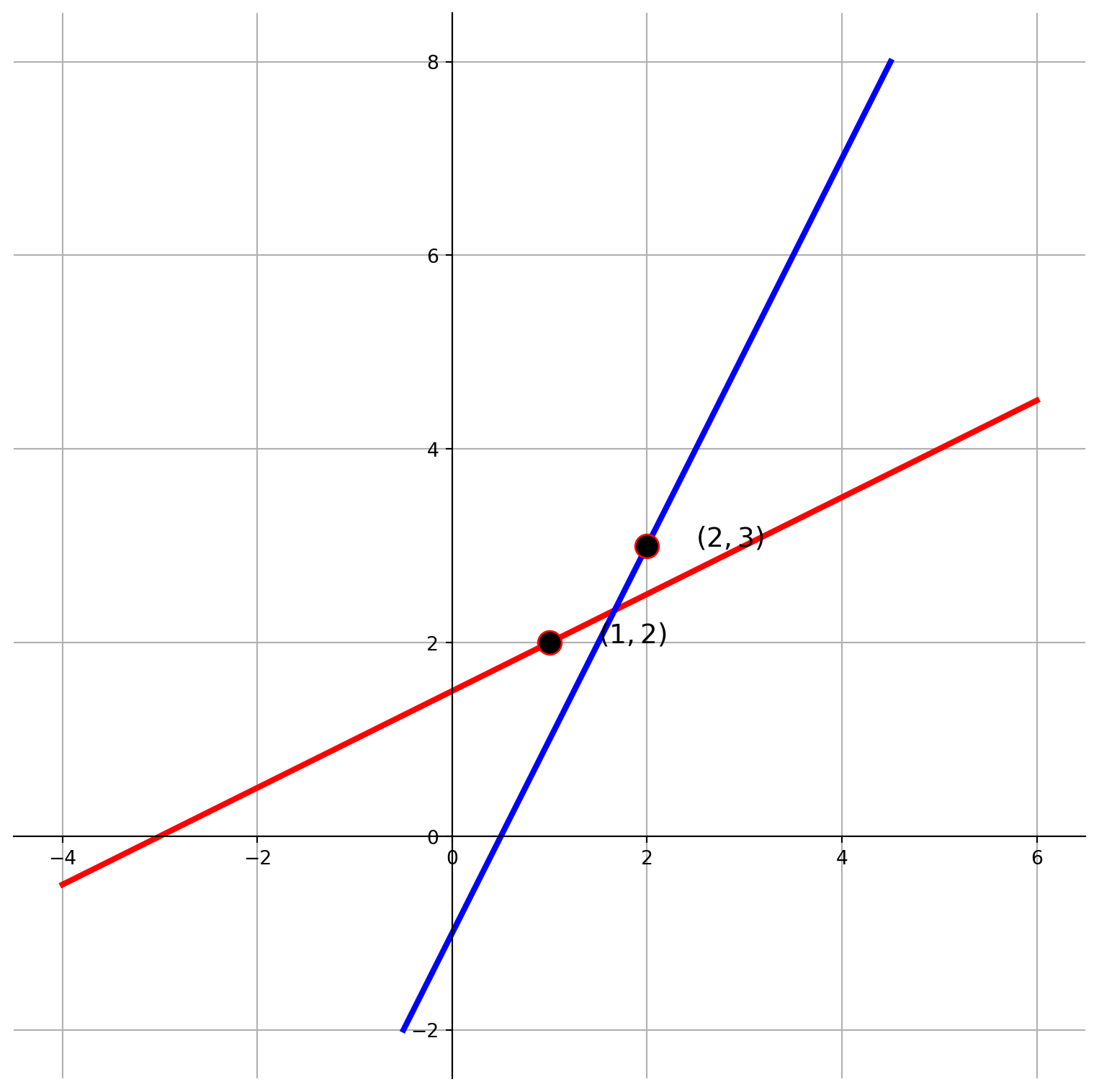
A Simple Linear Transformation
Now we know the parametric functions in \(\mathbb{R}^2\), we can show how a linear transformation acturally works on a line.
Let’s say, we perform linear transformation on a vector \((x, y)\),
\[ T\left(\begin{bmatrix} x \\ y \end{bmatrix}\right) = \begin{pmatrix} 3x - 2y \\ -2x + 3y \end{pmatrix} \] and substitute the parametric function into the linear operator.
\[ T\left(\begin{bmatrix} 4+t \\ 5+3t \end{bmatrix}\right) = \begin{pmatrix} 3(4+t) - 2(5+3t) \\ -2(4+t) + 3(5+3t) \end{pmatrix} = \begin{bmatrix} 2 - 3t \\ 7 + 7t \end{bmatrix} \]
The red line is transformed into blue line and point \((4, 5)\) transformed into \((2, 7)\)
p0 = np.array([[4], [5]])
v0 = np.array([[1], [3]])
p1 = np.array([[2], [7]])
v1 = np.array([[-3], [7]])
paraEqPlot(p0, v0, p1, v1)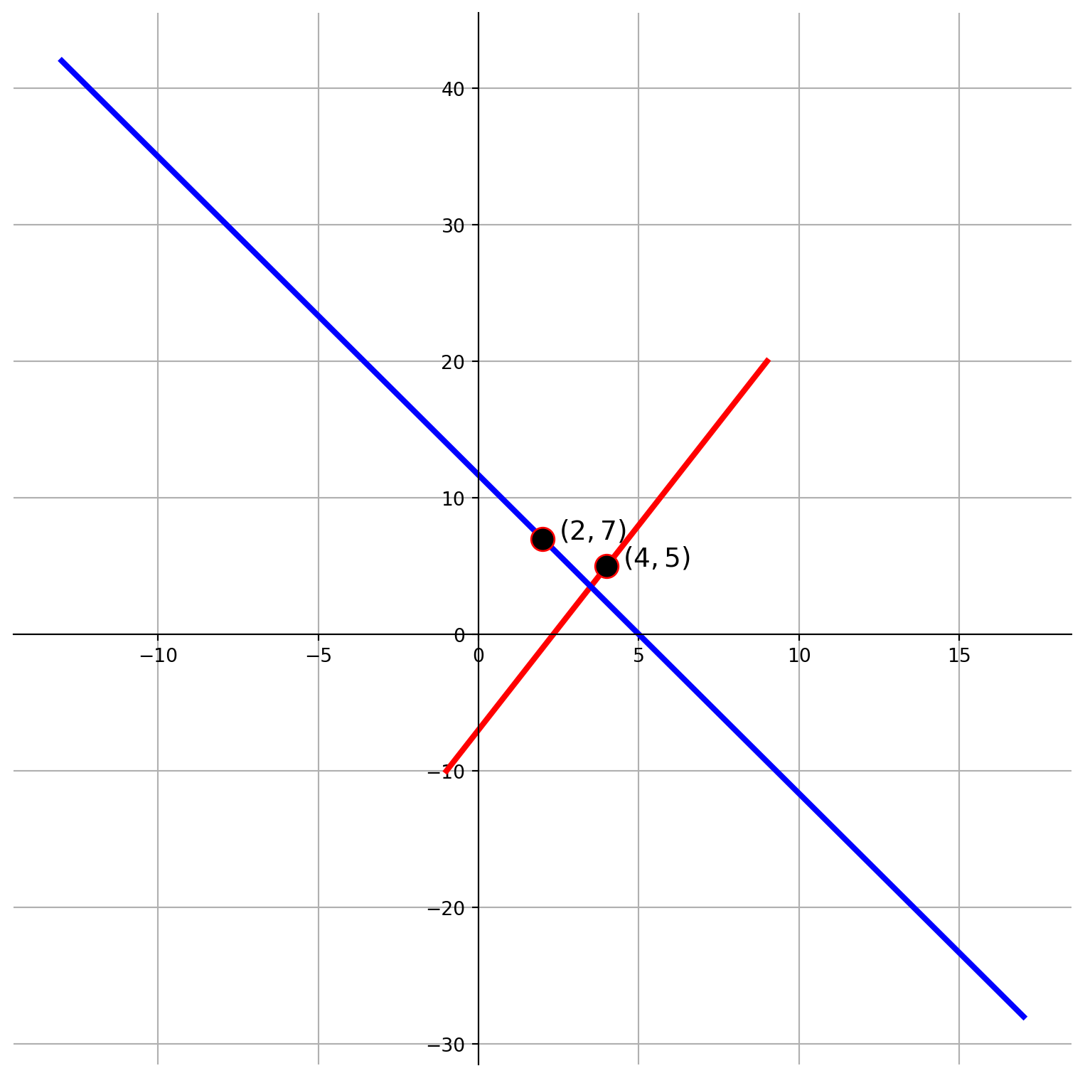
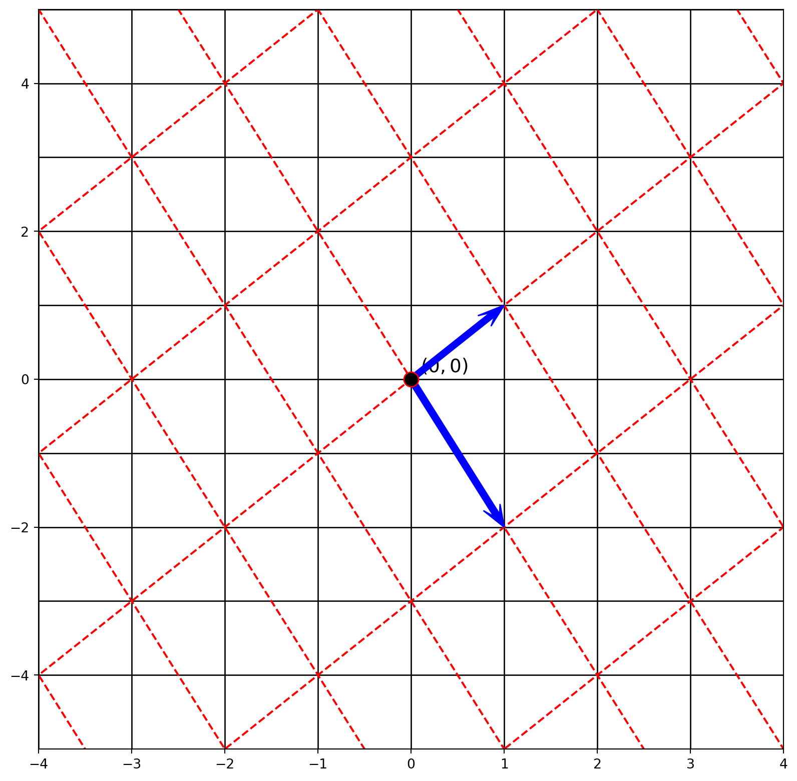
Visualization of Change of Basis
Change of basis is also a kind of linear transformation. Let’s create a grid.
u1, u2 = np.linspace(-5, 5, 10), np.linspace(-5, 5, 10)
U1, U2 = np.meshgrid(u1, u2)
We plot each row of \(U2\) again each row of \(U1\)
fig, ax = plt.subplots(figsize=(10, 10))
ax.plot(U1, U2, color="black")
ax.plot(U1.T, U2.T, color="black")
plt.show()
Let \(A\) and \(B\) be two bases in \(\mathbb{R}^3\)
\[ A = \left\{ \begin{bmatrix} 2 \\ 1 \end{bmatrix}, \ \begin{bmatrix} 1 \\ 1 \end{bmatrix} \right\} \\ B = \left\{ \begin{bmatrix} 3 \\ 2 \end{bmatrix}, \ \begin{bmatrix} 0 \\ -1 \end{bmatrix} \right\} \]
If we want to use basis \(A\) to represent \(B\), we can construct an augmented matrix like we did before.
\[ [A|B]= \left[ \begin{matrix} 2 & 1 & 3 & 0\\ 1 & 1 & 2 & -1 \end{matrix} \right] \]
AB = sy.Matrix([[2, 1, 3, 0], [1, 1, 2, -1]])
AB.rref()
\(\displaystyle \left( \left[\begin{matrix}1 & 0 & 1 & 1\\0 & 1 & 1 & -2\end{matrix}\right], \ \left( 0, \ 1\right)\right)\)
We find the transition matrix \(P_{A\leftarrow B}\) \[ [A|B]=[I|P_{A\leftarrow B}] \]
We can write
\[ \big[x\big]_A = P_{A\leftarrow B}\big[u\big]_B\\ \left[ \begin{matrix} x_1\\x_2 \end{matrix} \right] = \left[ \begin{matrix} 1 & 1\\1 & -2 \end{matrix} \right] \left[ \begin{matrix} u_1\\u_2 \end{matrix} \right]\\ \]
Therefore \[ x_1 = u_1+u_2\\ x_2 = u_1 - 2u_2 \]
Let’s plot original and transformed coordinates together.
u1, u2 = np.linspace(-10, 10, 21), np.linspace(-10, 10, 21)
U1, U2 = np.meshgrid(u1, u2)

fig, ax = plt.subplots(figsize=(10, 10))
ax.plot(U1, U2, color="black", lw=1)
ax.plot(U1.T, U2.T, color="black", lw=1)

X1 = U1 + U2
X2 = U1 - 2 * U2
ax.plot(X1, X2, color="red", ls="--")
ax.plot(X1.T, X2.T, color="red", ls="--")

ax.arrow(
    0,
    0,
    1,
    1,
    color="blue",
    width=0.07,
    length_includes_head=True,
    head_width=0.2,  # default: 3*width
    head_length=0.3,
    zorder=4,
    overhang=0.4,
)

ax.arrow(
    0,
    0,
    1,
    -2,
    color="blue",
    width=0.07,
    length_includes_head=True,
    head_width=0.2,  # default: 3*width
    head_length=0.3,
    zorder=4,
    overhang=0.4,
)

ax.text(0.1, 0.1, "$(0, 0)$", size=14)
ax.scatter(0, 0, s=120, zorder=5, ec="red", fc="black")

ax.axis([-4, 4, -5, 5])
plt.show()